cytorete: RNA regulon inference

cytorete infers regulons — a transcription factor with its weighted target set — from RNA alone, on the PIASO stack: promoter windows from the PIASO-data TSS annotation, sequence from the 2bit genome, motifs scanned with piaso.pp.scan_motifs, and edges kept only when the TF’s and the target’s COSG cell-type specificity profiles agree (piaso.tl.cospecificity_trans).

pip install cytorete        # pulls piaso-tools>=1.2.2, cosg, cytome

1. Inputs — all fetchable

import piaso

jaspar = piaso.data.fetch_jaspar()                # JASPAR CORE vertebrates MEME
twobit = piaso.data.fetch_2bit("hg38")            # genome sequence
piaso.data.fetch_genome("hg38")                   # TSS BED among the references
ds = piaso.data.load_dataset("sea_ad_mtg_20k_cytome",
                                      return_type="cytome")
piaso.settings.set_figure_params(style="cell")   # one house style across every figure

Human cortex, 20,000 nuclei, Subclass annotations — streamed from the .cytome, never loaded whole.

2. One call

import cytorete

cytorete.tl.inferRegulon(ds, "hg38", "Subclass",
                         jaspar_path=jaspar, twobit_path=twobit)

No TF list. That is deliberate, and it is the whole call: with tf_list=None the TF universe is every TF named in the motif database that is also expressed in this data, which is the only set that can produce an edge — a TF with no matrix cannot be scanned, and a TF absent from the data has no specificity profile to agree with anything. Passing a hand-picked list can only remove TFs that were usable, and it guarantees the network contains nothing you did not already believe.

What happened, from the run log:

[inferRegulon] genome=hg38 groupby='Subclass' gene universe = 36601 features
[inferRegulon] 740 TFs with motifs in the data
[inferRegulon] target_genes='cosg' → 4236 genes to scan (740 TFs always in)
[inferRegulon] 3141 genes with promoters (6342 intervals)
[cistrome]     scanning 795 PWMs (740 TFs) × 6342 promoter sequences (method=motif_bg)
[cistrome]     M = 740 TFs × 3141 genes, 175556 edges (7.55% density), 146 flat motifs dropped
[regulons]     412 global regulons (median 69 targets); per-cell-type regulons for 24 cell types
[regulonActivity]     scoring 412 regulons (layer=infog, pvalues=True)
[regulonSpecificity]  COSG on activity → 412 regulons × 24 cell types

Nine minutes, 20,000 nuclei, 412 regulons. Read the funnel: JASPAR2024 CORE vertebrates has 879 matrices, 740 of their TFs are expressed here, and target_genes='cosg' narrows the targets to the 4,236 genes that are specific to some cell type — scanning all 36,601 would spend most of the time on genes no regulon could claim. 146 matrices are dropped as too flat to discriminate, which is the scanner refusing to report a hit it cannot distinguish from background.

Everything is written back onto the object: per-cell activity in X_regulon (+ X_regulon_pval), the regulon store under the regulon key.

If you do want a shortlist

tf_list=["SOX9", "OLIG2", "SPI1", …] restricts the scan to those TFs. It is the right call when you have a hypothesis and want the p-values spent on it, and the wrong one when you are asking what the data contains.

3. Read the biology

cytorete.pl.regulonActivity(ds, groupby="Subclass")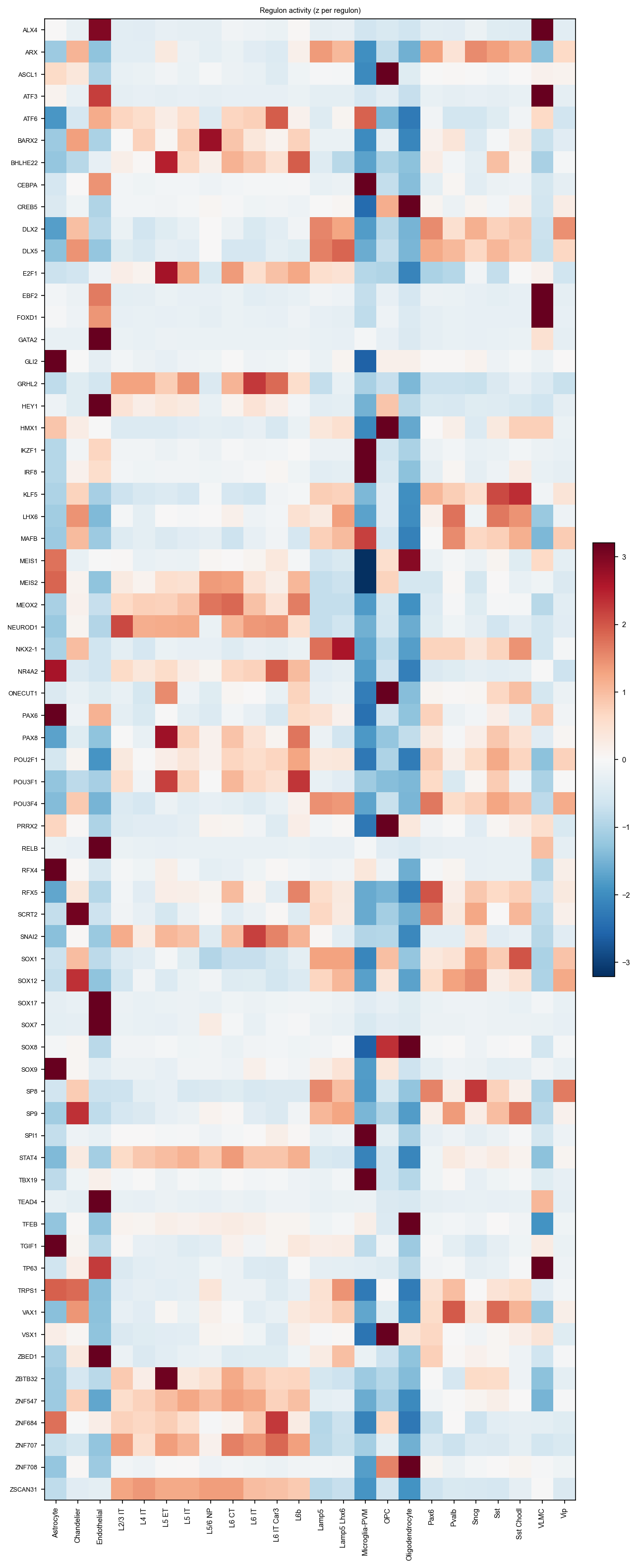

Specificity ranks, for each cell type, the regulons whose activity is most specific to it — COSG λ again, this time on the activity matrix rather than on expression. It is a two-step: compute, then plot.

spec = cytorete.tl.regulonSpecificity(ds, groupby="Subclass", copy=True)
cytorete.pl.regulonActivity(ds, groupby="Subclass", values="specificity")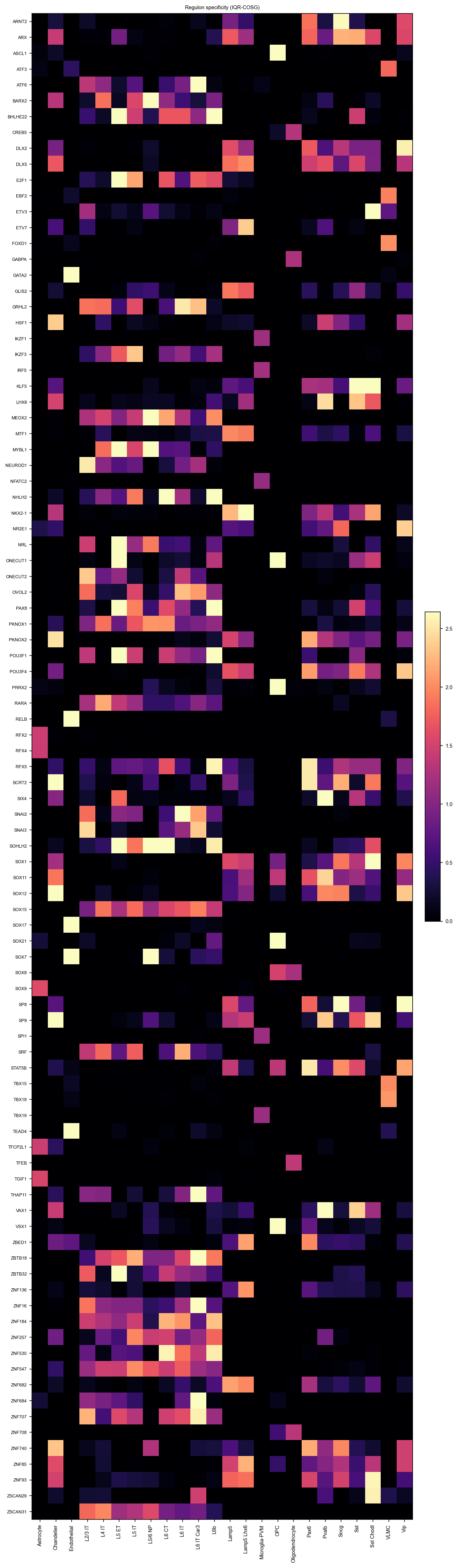

The top three regulons per cell type, from spec, with nothing supplied to the method beyond a count matrix and a subclass label:

cell type	top regulons
Astrocyte	SOX9, TGIF1, TFCP2L1
OPC	ASCL1, VSX1, PRRX2
Oligodendrocyte	TFEB, ZNF708, CREB5
Microglia-PVM	IRF5, IKZF1, SPI1
Endothelial	SOX17, GATA2, RELB
VLMC	TBX18, FOXD1, TBX15
Pvalb	SIX4, VAX1, LHX6
Sst	KLF5, VAX1, LHX6
Lamp5 Lhx6	NKX2-1, ETV7, ZNF85
Vip	SP8, DLX2, NR2E1
Sncg	SP8, ARNT2, ARX
L2/3 IT	NEUROD1, SNAI3, ONECUT2
L6b	POU3F1, BHLHE22, PAX8

Read the interneuron rows together. LHX6 and VAX1 head Pvalb and Sst, the two MGE-derived classes, and NKX2-1 heads Lamp5 Lhx6 — those three are the medial ganglionic eminence programme. SP8, DLX2 and ARX head Vip and Sncg, which are caudal ganglionic eminence. The method was told nothing about developmental origin; it recovered the MGE/CGE split from promoter sequence and specificity agreement alone. Glia and vasculature land equally cleanly: SOX9 in astrocytes, ASCL1 in OPCs, the SPI1/IRF5/IKZF1 myeloid trio in microglia, SOX17/GATA2 in endothelium, TBX18/FOXD1 in VLMC.

Also available: pl.regulonEmbedding (activity on the UMAP/spatial embedding), pl.regulonNetwork (the TF→target graph) and pl.regulonSpecificityScatter (§3c).

3a. Which cells are which

Every regulon panel below is drawn on this UMAP, so it is worth seeing the cell types on it first:

piaso.pl.plotEmbedding(ds, color="Subclass", basis="X_umap")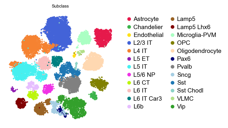

3b. Activity comes with a p-value

compute_pvalues=True is the default, so alongside X_regulon there is X_regulon_pval, from the same control-set null that PIASOscore uses:

import numpy as np
pvals = np.asarray(ds.embeddings["X_regulon_pval"])   # cells × regulons
names = md["names"]
j = names.index("CUX2")
(pvals[:, j] < 0.05).mean()          # fraction of cells with significant CUX2

Plot it beside the activity — the pair is more informative than either:

import numpy as np
P = np.asarray(ds.embeddings["X_regulon_pval"])
for tf in ["CUX2", "LHX6", "IRF8"]:
    j = names.index(tf)
    ds.cells[f"act_{tf}"] = np.asarray(ds.embeddings["X_regulon"])[:, j]
    ds.cells[f"nlp_{tf}"] = -np.log10(np.clip(P[:, j], 1e-300, 1))
ds.flush()

piaso.pl.plotEmbedding(ds, color="act_CUX2", basis="X_umap", vmin_pct=5, vmax_pct=95)
piaso.pl.plotEmbedding(ds, color="nlp_CUX2", basis="X_umap", vmin_pct=5, vmax_pct=95)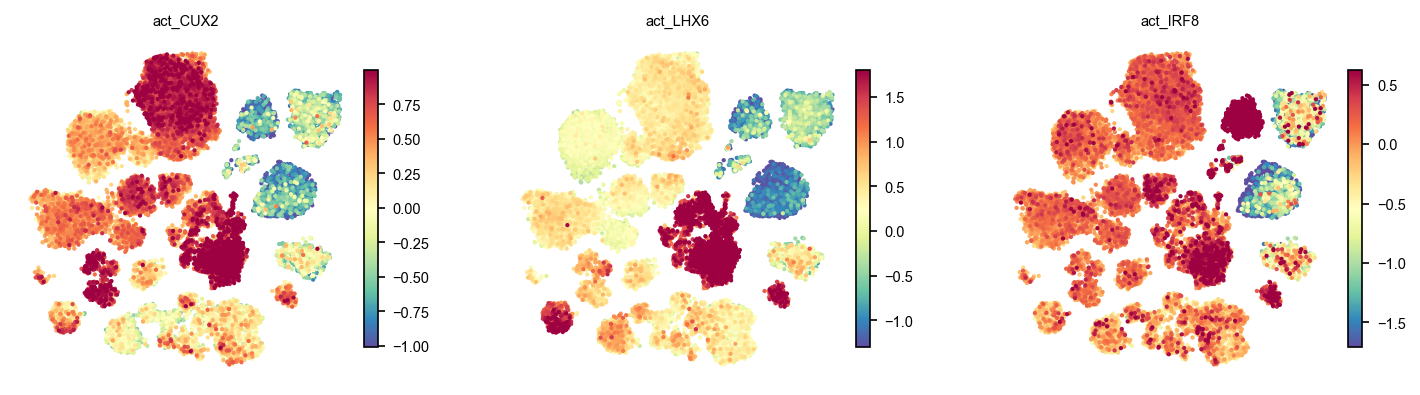

Read the two rows together. CUX2 and LHX6 reach −log10 p = 3.0 across their territories — and that is the ceiling, not a coincidence: with 1,000 control sets the smallest attainable p is 1/1001, so anything strongly significant piles up at exactly 3.0. The panels are saturated, which is the correct reading of “as significant as this test can report”.

IRF8 is the instructive one. Its activity is unmistakable in microglia, yet only 6% of cells clear p < 0.05 against 41% for the other two. Nothing is wrong: microglia are a small fraction of this dataset, the regulon is inactive nearly everywhere else, and a per-cell test asks whether this cell exceeds its own controls. A regulon can be highly specific and significant in few cells — specificity and per-cell significance are different questions, and the two rows let you see which one you are looking at.

Plot it like any other per-cell value:

for tf in ["CUX2", "LHX6", "IRF8"]:
    j = names.index(tf)
    ds.cells[f"negp_{tf}"] = -np.log10(np.clip(pvals[:, j], 1e-300, 1))
ds.flush()

piaso.pl.plotEmbedding(ds, color="negp_CUX2", basis="X_umap", vmin=0, vmax=3)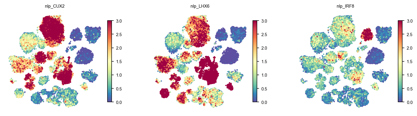

Significance is not a copy of activity. LHX6 reaches p < 0.05 in 41% of cells and IRF8 in 6% — IRF8’s regulon is small and confined to microglia, so almost everywhere else it is indistinguishable from its control sets, which is the correct answer rather than a weak one. Reading the activity panel alone would suggest a graded signal across the section; the p-value says where that gradient is worth interpreting.

The p-value is permutation-based, so it floors at 1/(n_permutations+1) — -log10(p) saturates at 3.0 with the default 1,000 control sets, and values at the ceiling are “as significant as this test can report”, not “more significant than the others there.”

3c. The other three views

cytorete.pl has four plot functions; the heatmap above is one. The other three answer different questions on the same result.

Where is a regulon active? — activity on any embedding:

cytorete.pl.regulonEmbedding(ds, regulons=["CUX2", "LHX6", "IRF8"],
                             basis="X_umap", key="X_regulon")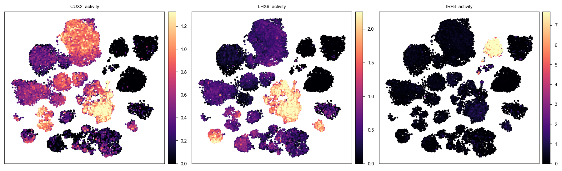

Three regulons, three territories, none of them supplied to the method: CUX2 in upper-layer excitatory neurons, LHX6 in MGE-derived interneurons, IRF8 in microglia.

What is in a regulon? — the TF and its targets:

cytorete.pl.regulonNetwork(ds, tf="CUX2", max_targets=20)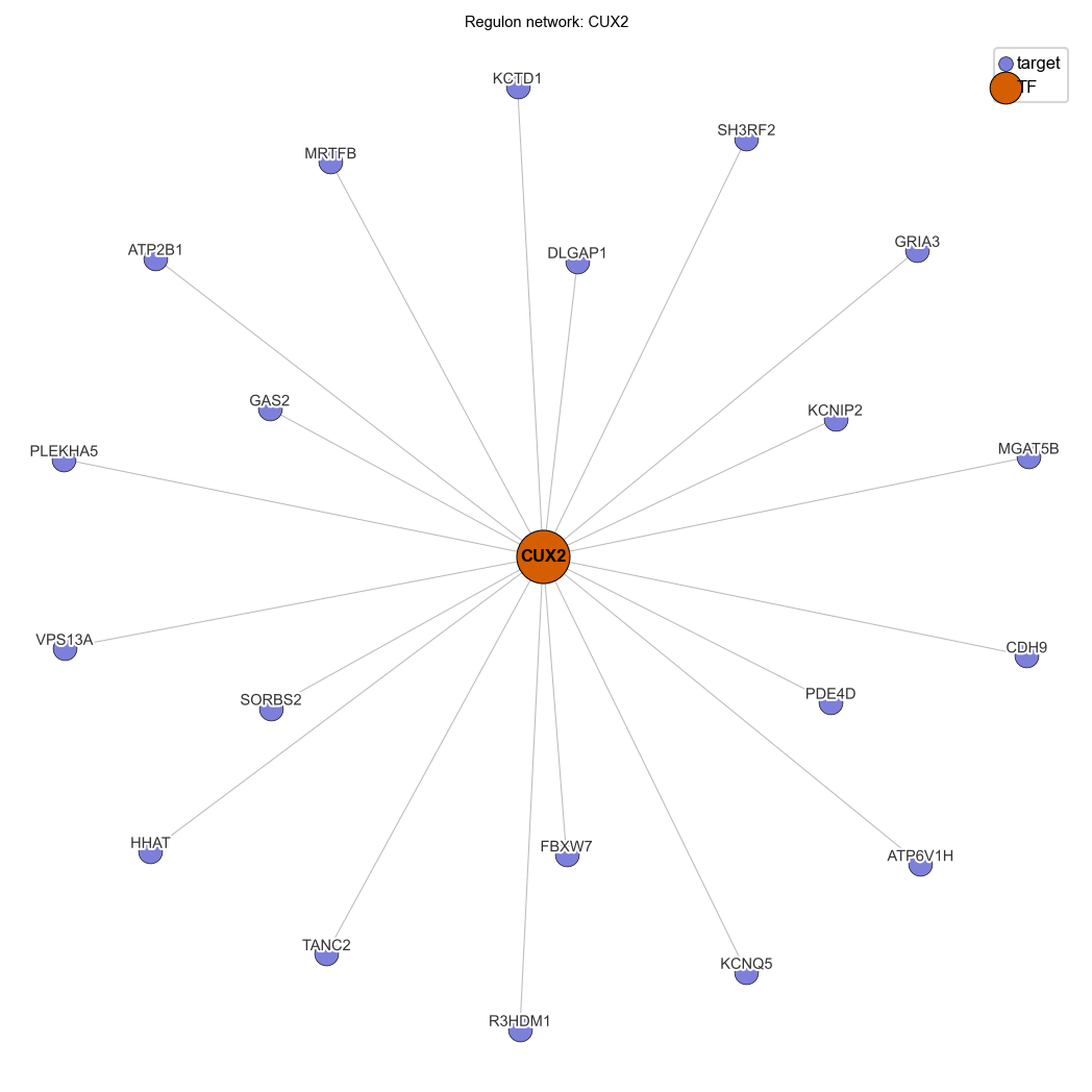

Target names are drawn by default (label_targets=False for dense multi-TF layouts). CUX2’s here are synaptic and channel genes — GRIA3, KCNQ5, DLGAP1, CDH9 — which is the sanity check worth doing before believing a regulon.

Is the TF’s own expression driving it? — one panel per cell type, one dot per TF, regulon-activity specificity against the specificity of the TF’s own expression:

cytorete.pl.regulonSpecificityScatter(ds, groupby="Subclass", key="X_regulon")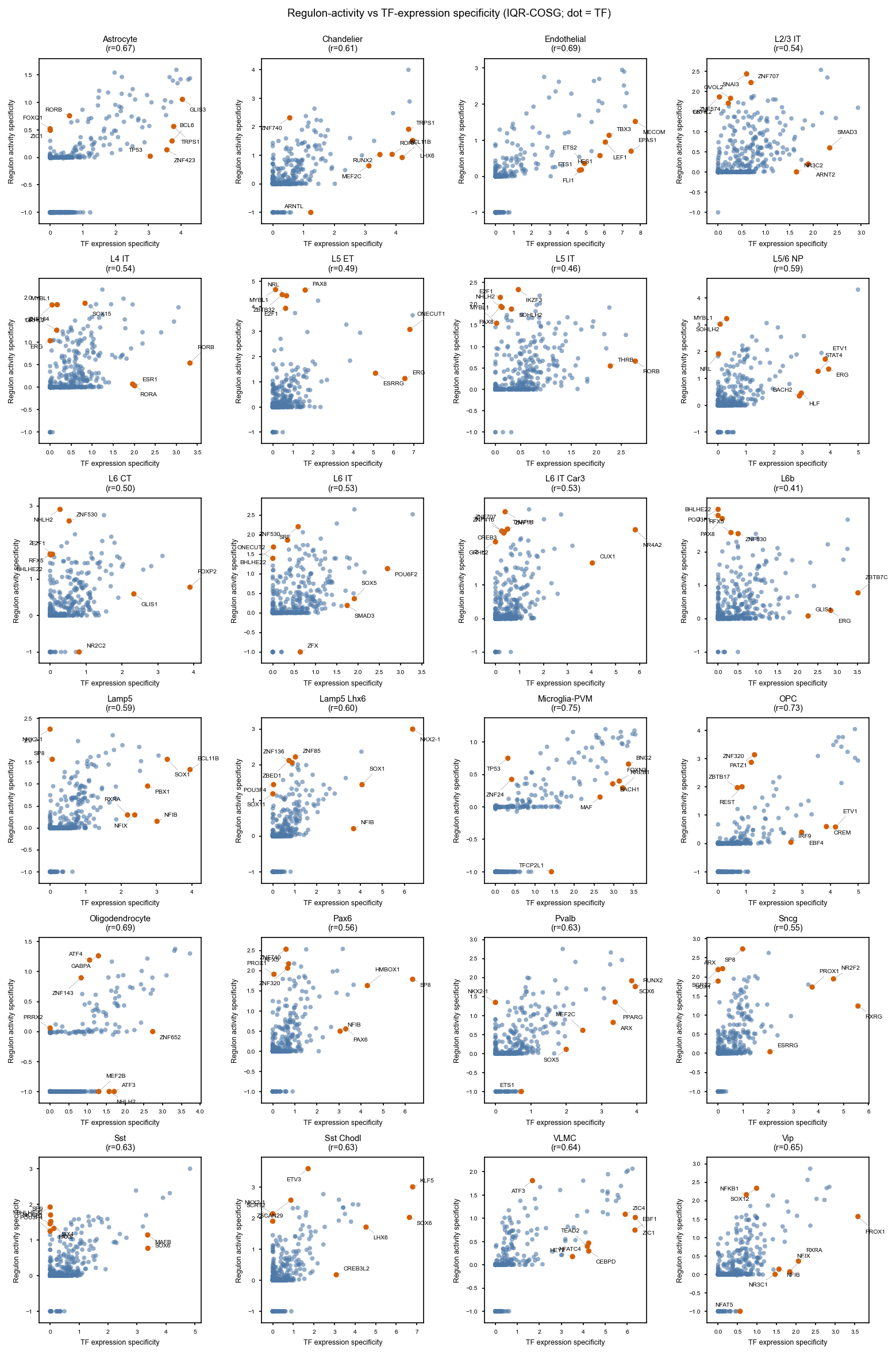

key="X_regulon" is worth passing explicitly: the function defaults to "X_grn", which is what inferGRN writes, not what inferRegulon does.

The two axes are the question. A TF high on both is specific and expressed here, which is the easy case. A TF high on the y-axis and low on the x-axis is one whose targets are coherent in this cell type without the TF’s own transcript being distinctive — the case a co-expression method cannot see, and the reason the edges come from promoter sequence rather than from the TF’s expression. It is also the failure mode a recent Jacobian benchmark documented for dynamical GRN inference: recovery biased toward target genes over regulators, because TFs are lowly and noisily expressed.

What is not here yet

This release infers regulons from RNA. The multiome route — cistromes built from accessible peaks rather than promoter windows alone, using paired RNA + ATAC — is in development and will be released separately. Its entry points (inferGRN, inferTFActivity) exist in the package today and raise an ImportError naming what they need, so import cytorete behaves the same either way.

4. How the edges are decided

1. Promoter cistrome — strand-aware windows (−1000/+500 around each TSS; alternative promoters kept separate) scanned against the motif DB with a per-motif background model, giving TF → gene motif support.
2. Trans co-specificity — each motif-supported pair is scored by the cosine agreement of the TF’s and target’s COSG specificity profiles across your groupby cell types; positive-sign edges above the threshold survive, per cell type.
3. Regulon assembly keeps TFs with at least min_targets surviving targets. NES pruning is available — cistrome_method="nes" switches the cistrome to an RcisTarget-style normalised enrichment score with nes_threshold — but it is not the default; motif_bg is.
4. Activity is piaso.tl.score (PIASOscore), PIASO’s own gene-set scorer, not AUCell: for each cell it scores the regulon against size- and expression-matched control gene sets drawn from the same data, so a large regulon and a small one are comparable. Because the controls give a null, compute_pvalues=True (the default) also writes a per-cell p-value beside the score.

Works identically on an AnnData — the same run, in an AnnData does the whole chain on the h5ad of this dataset and reports where each result lands. On a cytome every stage streams.

The motif engine itself — PWMs, backgrounds, p-value→score thresholds — is documented in the Motif analysis tutorial. Its §10 is worth reading alongside this page: it measures two motif-only ways of asking “which TFs’ motifs sit in this cell type’s markers”, finds that both fail, and shows why the co-specificity step on this page is what makes the answer about a TF rather than about a motif family.