Spatial: Stereo-seq whole embryo

MOSTA series — chapter 1 of 4: One section into a cytome

Builds mosta_e16.cytome from a single E16.5 section, and gets the orientation right before anything is drawn on it.

Chapter 2: Eight stages in one embedding →

Stereo-seq captures whole organisms at subcellular bin resolution — the files are big, which is exactly cytome territory. This tutorial uses the MOSTA mouse organogenesis atlas (Chen et al., Cell 2022): one E16.5 sagittal section, 121,767 bins × 28,204 genes, with the paper’s organ annotations.

1. Data (CNGB, direct download, ~4.8 GB)

curl -O https://ftp.cngb.org/pub/SciRAID/stomics/STDS0000058/stomics/E16.5_E1S1.MOSTA.h5ad

Smaller sections from the same atlas work identically (e.g. Mouse_brain.h5ad, ~1 GB). The human embryogenesis counterpart (HESTA, CS12–CS23) is browsed at db.cngb.org/hesta; its per-section downloads go through the STOmics DB.

2. One conversion, everything indexed

import anndata as ad
import cytome
import piaso

a = ad.read_h5ad("E16.5_E1S1.MOSTA.h5ad")      # obsm['spatial'], obs['annotation']
ds = cytome.from_anndata(a, output="mosta_e16.cytome")
piaso.settings.set_figure_params(style="cell")   # one house style across every figure

90 seconds, 1.55 GB on disk — and obsm['spatial'] became both the spatial embedding and the R*-tree coordinate index (all 121,767 bins queryable by rectangle). From here the h5ad is no longer needed.

3. The embryo, as delivered

piaso.pl.plotEmbedding(ds, color="annotation", basis="spatial",
                       point_size=0.8, legend_loc="right", legend_ncol=2)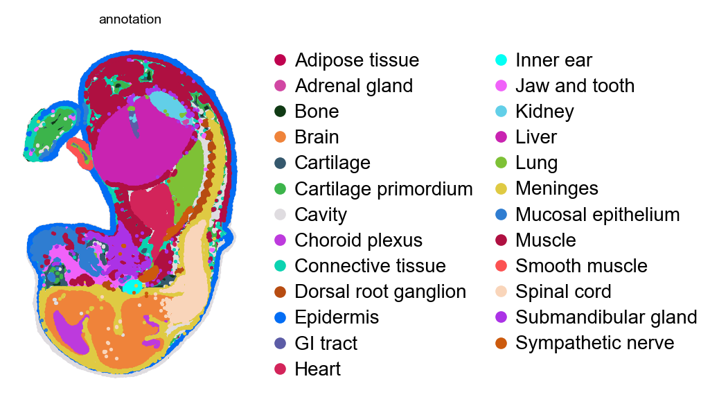

The embryo arrives head down. Nothing is wrong with the coordinates — MOSTA stores them in the orientation the section was captured in — but every figure after this one reads better with the head up, which is the next section.

4. Orient the section

Sections land on the chip in arbitrary orientation. piaso.pp rotates the coordinates about their centroid — directly on the cytome, no AnnData round-trip.

This section arrives head down, as section 3 shows, so it does need correcting — by 180°. Before doing that irreversibly, it is worth seeing what the function does to a frame you can throw away.

Demonstration first. Rotate a copy by 90°, leaving the delivered coordinates untouched. The angle is arbitrary; the point is to see the call work and to keep the original beside it:

import numpy as np
import matplotlib.pyplot as plt

# Conversion prefixes obsm keys with the modality, so `spatial` is stored as
# `RNA_spatial`. `ds.list_embeddings()` shows the names actually present.
# work on a copy so the frame every other section plots stays put
ds.add_embedding("spatial_demo",
                 np.asarray(ds.embeddings["RNA_spatial"]).astype(np.float32))
# backup_spatial_key is what creates `spatial_original`; without it the
# rotation happens in place and there is nothing left to compare against.
piaso.pp.rotateSpatialCoordinates(ds, angle_degrees=90,
                                  spatial_key="spatial_demo",
                                  backup_spatial_key="spatial_original")

fig, axes = plt.subplots(1, 2, figsize=(15, 7))
piaso.pl.plotEmbedding(ds, color="annotation", basis="spatial_original",
                       ax=axes[0], show=False, legend_loc=None)
axes[0].set_title("as delivered — head down")
piaso.pl.plotEmbedding(ds, color="annotation", basis="spatial_demo",
                       ax=axes[1], show=False, legend_loc=None)
axes[1].set_title("rotateSpatialCoordinates(angle_degrees=90)")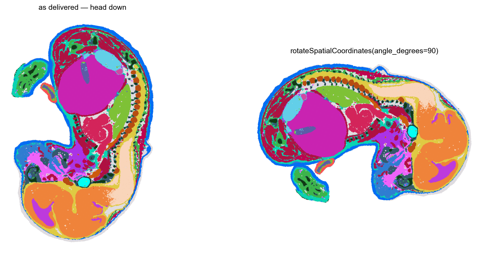

The rotation is written into the file, and when the rotated embedding is the spatial one the spatial_coords R*-tree is rebuilt in the same call — so cells_in_region (below) keeps agreeing with what you plot. spatial_key resolves the same way plotting’s basis= does; backup_spatial_key= keeps the original one assignment away; clockwise=True flips the direction.

Rotating in place when you did not need to is the mistake to avoid: every figure downstream inherits it, and there is no warning because nothing is wrong with the coordinates — only with the orientation you chose. Rotate a copy, look at it, and only then decide.

Now the correction. The demo above was 90° on a throwaway copy; the fix this section actually needs is 180° on spatial itself, which turns the delivered head-down frame the right way up. From here every figure on this page is head up, because they all read spatial and spatial has been rotated:

piaso.pp.rotateSpatialCoordinates(ds, angle_degrees=180, spatial_key="spatial",
                                  backup_spatial_key="spatial_delivered")

piaso.pl.plotEmbedding(ds, color="annotation", basis="spatial",
                       point_size=0.8, legend_loc="right", legend_ncol=2)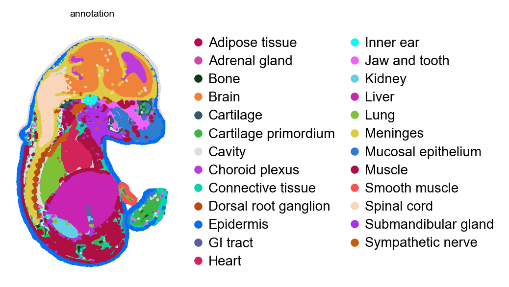

backup_spatial_key keeps the delivered frame under spatial_delivered, so the rotation is reversible and the original is still there to compare against.

A path works too, if the dataset is not already open. Note the different key: rotating spatial again here would turn the section by another 180° and put the head back where it started — the rotation is written to the file, so a second call composes with the first rather than replacing it.

piaso.pp.rotateSpatialCoordinates("mosta_e16.cytome", angle_degrees=180,
                                  spatial_key="spatial_demo")

The same call takes an AnnData (rotateSpatialCoordinates(adata, ...), reading obsm[spatial_key]), where inplace=False returns a rotated copy. On a cytome inplace=False raises instead: a file cannot pretend to be a copy.

5. Zoom by coordinates

The indexed rectangle query returns the row indices of the bins in that window. Coordinates and labels both come off the cytome directly, so the zoom needs no AnnData and no matrix read:

# a window around the head, taken from where the Brain bins actually are
brain = ds.embeddings["RNA_spatial"][np.asarray(ds.cells["annotation"]) == "Brain"]
x0, x1 = np.percentile(brain[:, 0], [1, 99])
y0, y1 = np.percentile(brain[:, 1], [1, 99])

sel = ds.cells_in_region(x=(x0, x1), y=(y0, y1))
piaso.pl.plotEmbedding(ds, color="annotation", basis="spatial", cell_mask=sel)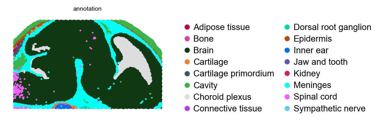

That window returns 28,881 bins spanning 19 annotated types — brain filling it, with choroid plexus, meninges, inner ear and the head skeleton around the edge. Deriving the rectangle from the label rather than typing coordinates is what makes it reproducible on a section you have not seen.

If a registered ssDNA image is available for your section, store it with ds.add_spatial_image(...) and the same window drives ds.spatial_images.crop(...) — one rectangle, cells and pixels — with image=True overlays on every plot above (see the Xenium tutorial).

6. Where to take it

From the same cytome, streaming INFOG → SVD → GDR and marker detection run in bounded working memory — the full expression matrix is never loaded (see GDR at scale), and the regulon workflow in cytorete applies directly — the MOSTA paper’s own organ-identity regulon analysis is a natural exercise.